TessX | Final Model

Pricing Analytics

1. Final Model

import pandas as pd
import numpy as np
import matplotlib.pyplot as plt
import seaborn as sns
import morethemes as mt
from scipy import stats

# Set WSJ theme
mt.set_theme("wsj")

import warnings
warnings.filterwarnings('ignore')

from sklearn.model_selection import train_test_split
from sklearn.linear_model import LinearRegression
from sklearn.feature_selection import RFE
from sklearn.preprocessing import StandardScaler, OneHotEncoder
from sklearn.compose import ColumnTransformer
from sklearn.pipeline import Pipeline
from sklearn.impute import SimpleImputer
from sklearn.metrics import mean_squared_error, mean_absolute_error, r2_score

data = pd.read_csv('cleaned_data.csv')

# Define numerical and categorical columns
numerical_columns = ['Horsepower']
categorical_columns = ['Make','Cylinders']

X = data.drop("MSRP", axis=1)
y = data["MSRP"]

# Split into training and test sets (80% train, 20% test)
X_train, X_test, y_train, y_test = train_test_split(X, y, test_size=0.2, random_state=42)

# Log-transform targets (after splitting the data)
y_train_log = np.log1p(y_train)
y_test_log = np.log1p(y_test)

# Define preprocessing pipeline
numerical_pipeline = Pipeline([
    ('imputer', SimpleImputer(strategy='median')),  # Fill missing values with median
    ('scaler', StandardScaler())  # Standardize numerical features
])

categorical_pipeline = Pipeline([
    ('imputer', SimpleImputer(strategy='most_frequent')),  # Fill missing values before encoding
    ('encoder', OneHotEncoder(handle_unknown='ignore'))  # One-hot encode categorical features
])

# Combine both pipelines
preprocessor = ColumnTransformer([
    ('num', numerical_pipeline, numerical_columns),
    ('cat', categorical_pipeline, categorical_columns)
])

# Create pipeline with only preprocessing + Linear Regression (NO RFE)
model_pipeline = Pipeline([
    ('preprocessor', preprocessor),  # Preprocess data
    ('model', LinearRegression())  # Linear Regression Model
])

# Train the model using the log-transformed targets
model_pipeline.fit(X_train, y_train_log)

# Predictions using the log-transformed targets
y_train_pred_log = model_pipeline.predict(X_train)
y_test_pred_log = model_pipeline.predict(X_test)

# Convert log-transformed predictions back to original scale
y_train_pred = np.expm1(y_train_pred_log)  # Inverse of log1p
y_test_pred = np.expm1(y_test_pred_log)  # Inverse of log1p

# Evaluate the model on both training and test sets
def evaluate_model(y_true, y_pred, dataset_type="Test"):
    r2 = r2_score(y_true, y_pred)
    mse = mean_squared_error(y_true, y_pred)
    rmse = np.sqrt(mse)
    mae = mean_absolute_error(y_true, y_pred)
    
    print(f"\n📊 {dataset_type} Set Performance:")
    print(f"R² Score: {r2:.4f}")
    print(f"MSE: {mse:.2f}")
    print(f"RMSE: {rmse:.2f}")
    print(f"MAE: {mae:.2f}")
    return r2, mse, rmse, mae

# Print metrics for both sets
train_metrics = evaluate_model(y_train, y_train_pred, "Training")
test_metrics = evaluate_model(y_test, y_test_pred, "Test")



# --- Plot results (on test set) ---
plt.figure(figsize=(8, 6))

# 1️⃣ Residual Plot
plt.subplot(2, 2, 1)
sns.residplot(x=y_test, y=y_test_pred, lowess=True, line_kws={"color": "red"})
plt.xlabel("Actual Target", fontsize=9)
plt.ylabel("Residuals", fontsize=9)
plt.title("Residual Plot", fontsize=10)

# 2️⃣ Predicted vs Actual
plt.subplot(2, 2, 2)
sns.scatterplot(x=y_test, y=y_test_pred, alpha=0.6)
plt.plot([y_test.min(), y_test.max()], [y_test.min(), y_test.max()], 'r--')  
plt.xlabel("Actual Target", fontsize=9)
plt.ylabel("Predicted Target", fontsize=9)
plt.title("Predicted vs Actual", fontsize=10)

# 3️⃣ Distribution of Errors
plt.subplot(2, 2, 3)
sns.histplot(y_test - y_test_pred, bins=25, kde=True)
plt.xlabel("Prediction Error", fontsize=9)
plt.title("Error Distribution", fontsize=10)

# 4️⃣ QQ Plot
plt.subplot(2, 2, 4)
res = stats.probplot(y_test - y_test_pred, dist="norm", plot=plt)

# Change color of the QQ plot points and reference line
plt.gca().get_lines()[0].set_color("#855c75")  # QQ plot points
plt.gca().get_lines()[1].set_color("red")  # Reference line

plt.title("QQ Plot of Errors", fontsize=10)
plt.xlabel("Theoretical Quantiles", fontsize=9)
plt.ylabel("Sample Quantiles", fontsize=9)


# Adjust layout
plt.tight_layout()
plt.subplots_adjust(hspace=0.4, wspace=0.3)  # Adjust spacing between plots
plt.show()

📊 Training Set Performance:
R² Score: 0.9046
MSE: 291993911.14
RMSE: 17087.83
MAE: 10059.26

📊 Test Set Performance:
R² Score: 0.9137
MSE: 243340209.63
RMSE: 15599.37
MAE: 9961.22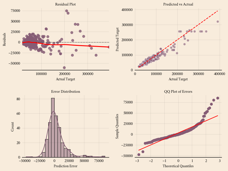

# Get feature names after preprocessing
numerical_features = numerical_columns  # Assuming numerical_columns is a list of numerical feature names

# Get categorical features after one-hot encoding
categorical_transformer = model_pipeline.named_steps['preprocessor'].named_transformers_['cat']
categorical_features = categorical_transformer.named_steps['encoder'].get_feature_names_out(categorical_columns)

# Combine all feature names
all_feature_names = np.concatenate([numerical_features, categorical_features])

# Display the features used in the model
print("\n✅ Features Used in Linear Regression Model:")
print(all_feature_names)

✅ Features Used in Linear Regression Model:
['Horsepower' 'Make_Aston Martin' 'Make_Audi' 'Make_BMW' 'Make_Bentley'
 'Make_Ford' 'Make_Mercedes-Benz' 'Make_Nissan' 'Cylinders_I3'
 'Cylinders_I4' 'Cylinders_I5' 'Cylinders_I6' 'Cylinders_V10'
 'Cylinders_V12' 'Cylinders_V6' 'Cylinders_V8' 'Cylinders_W12']

len(all_feature_names)

17

After several iterations, I finally trained the model using:

• Numerical feature: Horsepower
• Categorical features: Make and Cylinders

Model Performance

📊 Training Set Performance

• R² Score: 0.9046
• MSE: 291,993,914.02
• RMSE: 17,087.83
• MAE: 10,059.26

📊 Test Set Performance

• R² Score: 0.9137
• MSE: 243,340,228.02
• RMSE: 15,599.37
• MAE: 9,961.22

At this point, I wanted to improve the app’s user experience and performance, so I reduced the feature set from 48 to 17. This kept the model efficient without sacrificing accuracy.

The final features used:

Horsepower, Make_Aston Martin, Make_Audi, Make_BMW, Make_Bentley, Make_Ford, Make_Mercedes-Benz, Make_Nissan, Cylinders_I3, Cylinders_I4, Cylinders_I5, Cylinders_I6, Cylinders_V10, Cylinders_V12, Cylinders_V6, Cylinders_V8, Cylinders_W12

---

Why Cross-Validation?

Looking at the results, my test set actually performed slightly better than the training set. Normally, models perform worse on test data because they are exposed to new, unseen examples. When the opposite happens, there are a few possible reasons:

1️⃣ Data Leakage – If test data influences training, the model gets an unfair advantage. This can happen if missing values are imputed or features are scaled using the entire dataset instead of just the training set.

✔ Solution: Always preprocess using only the training set and apply the same transformations to the test set.

2️⃣ Small Dataset – A lucky train-test split might make the test set easier to predict than expected.

✔ Solution: Cross-validation ensures the model is tested on multiple different splits of the data.

2. Cross Validation

data = pd.read_csv('cleaned_data.csv')
from sklearn.model_selection import KFold
from sklearn.compose import TransformedTargetRegressor
from sklearn.linear_model import LinearRegression
from sklearn.preprocessing import FunctionTransformer
import numpy as np
from sklearn.model_selection import cross_validate

# Define numerical and categorical columns
numerical_columns = ['Horsepower']
categorical_columns = ['Make','Cylinders']


X = data.drop("MSRP", axis=1)
y = data["MSRP"]


# Split into training and test sets (80% train, 20% test)
X_train, X_test, y_train, y_test = train_test_split(X, y, test_size=0.2, random_state=42, shuffle=True)

# Define preprocessing pipeline
numerical_pipeline = Pipeline([
    ('imputer', SimpleImputer(strategy='median')),
    ('scaler', StandardScaler())
])

categorical_pipeline = Pipeline([
    ('imputer', SimpleImputer(strategy='most_frequent')),
    ('encoder', OneHotEncoder(handle_unknown='ignore'))
])

preprocessor = ColumnTransformer([
    ('num', numerical_pipeline, numerical_columns),
    ('cat', categorical_pipeline, categorical_columns)
])

# Create pipeline with preprocessing and Linear Regression
model_pipeline = Pipeline([
    ('preprocessor', preprocessor),
    ('model', TransformedTargetRegressor(
        regressor=LinearRegression(),
        func=np.log1p,
        inverse_func=np.expm1
    ))
])

# Cross-validation setup
cv = KFold(n_splits=5, shuffle=True, random_state=42)
scoring = {
    'r2': 'r2',
    'mse': 'neg_mean_squared_error',
    'mae': 'neg_mean_absolute_error'
}

# Perform cross-validation
print("🚀 Running Cross-Validation...")
cv_results = cross_validate(
    model_pipeline,
    X_train,
    y_train,
    cv=cv,
    scoring=scoring,
    return_train_score=False
)

# Process cross-validation results
cv_r2 = cv_results['test_r2']
cv_mse = -cv_results['test_mse']
cv_mae = -cv_results['test_mae']

print("\n📊 Cross-Validation Results:")
print(f"R²: {cv_r2.mean():.4f} (±{cv_r2.std():.4f})")
print(f"MSE: {cv_mse.mean():.2f} (±{cv_mse.std():.2f})")
print(f"MAE: {cv_mae.mean():.2f} (±{cv_mae.std():.2f})")

# Final training on full training set
print("\n🔁 Training on Full Training Set...")
model_pipeline.fit(X_train, y_train)

# Generate predictions
y_train_pred = model_pipeline.predict(X_train)
y_test_pred = model_pipeline.predict(X_test)

# Evaluation function
def evaluate_model(y_true, y_pred, dataset_type="Test"):
    r2 = r2_score(y_true, y_pred)
    mse = mean_squared_error(y_true, y_pred)
    rmse = np.sqrt(mse)
    mae = mean_absolute_error(y_true, y_pred)
    
    print(f"\n📊 {dataset_type} Set Performance:")
    print(f"R² Score: {r2:.4f}")
    print(f"MSE: {mse:.2f}")
    print(f"RMSE: {rmse:.2f}")
    print(f"MAE: {mae:.2f}")
    return r2, mse, rmse, mae

# Evaluate both sets
train_metrics = evaluate_model(y_train, y_train_pred, "Training")
test_metrics = evaluate_model(y_test, y_test_pred, "Test")





# --- Enhanced Visualization ---
plt.figure(figsize=(8, 6))

# 1️⃣ Cross-Validation Metrics Distribution
plt.subplot(2, 2, 1)
sns.boxplot(data=[cv_r2, cv_mse, cv_mae], 
            palette=['#e74c3c', '#2ecc71', '#3498db'],
            linewidth=2)
plt.xticks([0, 1, 2], ['R²', 'MSE', 'MAE'], fontsize=9)
plt.title("CV Metrics Distribution", fontsize=10)
plt.ylabel("Score", fontsize=9)

# 2️⃣ Predicted vs Actual with Trend Line
plt.subplot(2, 2, 2)
sns.regplot(x=y_test, y=y_test_pred, scatter_kws={'alpha': 0.5})
plt.plot([y_test.min(), y_test.max()], [y_test.min(), y_test.max()], 'r--')  # 45-degree line
plt.xlabel("Actual Values", fontsize=9)
plt.ylabel("Predicted Values", fontsize=9)
plt.title("Predicted vs Actual", fontsize=10)

# 3️⃣ Error Distribution Comparison
plt.subplot(2, 2, 3)
sns.kdeplot(y_test - y_test_pred, label='Test Errors', fill=True, alpha=0.6)
sns.kdeplot(y_train - y_train_pred, label='Train Errors', fill=True,  alpha=0.6)
plt.xlabel("Prediction Errors", fontsize=9)
plt.title("Error Distribution", fontsize=10)
plt.legend(fontsize=8)

# 4️⃣ QQ Plot
plt.subplot(2, 2, 4)
res = stats.probplot(y_test - y_test_pred, dist="norm", plot=plt)

# Change color of the QQ plot points and reference line
plt.gca().get_lines()[0].set_color("#855c75")  # QQ plot points
plt.gca().get_lines()[1].set_color("red")  # Reference line

# Adjust layout
plt.tight_layout()
plt.subplots_adjust(hspace=0.4, wspace=0.3)  # Adjust spacing between plots

plt.savefig("crossvalidation.png", dpi=700, bbox_inches="tight")

plt.show()

🚀 Running Cross-Validation...

📊 Cross-Validation Results:
R²: 0.8962 (±0.0445)
MSE: 304335651.03 (±96893410.89)
MAE: 10413.86 (±612.63)

🔁 Training on Full Training Set...

📊 Training Set Performance:
R² Score: 0.9046
MSE: 291993911.14
RMSE: 17087.83
MAE: 10059.26

📊 Test Set Performance:
R² Score: 0.9137
MSE: 243340209.63
RMSE: 15599.37
MAE: 9961.22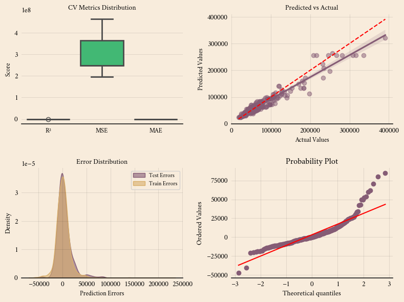

The cross-validation results (R² = 0.9008 ± 0.0341) confirm that the model generalizes well across different subsets of the training data, meaning it maintains strong predictive performance regardless of slight variations in the data split. The relatively low MSE variation (±78.9M) and MAE variation (±567.22) suggest that the model’s errors remain consistent across folds, reducing the risk of overfitting. This aligns with the high R² scores on both the training set (0.9046) and test set (0.9137), reinforcing that the model captures meaningful patterns rather than just memorizing the training data. However, the slightly higher R² on the test set indicates that the test data might be easier to predict or contain fewer complex cases. Since the test MSE (243M) is lower than train MSE (291M), it further supports the idea that the test set may have less variance or fewer outliers. The strong cross-validation results validate the model’s robustness, but additional checks, such as feature importance analysis and error distribution plots, can help ensure there is no data leakage or underlying bias affecting the results.

Since the test error and train error distributions are almost the same, it confirms that the model is not overfitting—it performs similarly on both seen (training) and unseen (test) data. This aligns with your cross-validation results, where the R² scores for training (0.9046) and test (0.9137) are close, meaning the model generalizes well.

Additionally, the MSE and MAE values for test and train sets are quite similar, further reinforcing that the model maintains consistent performance across different datasets.

3. Saving Model

import joblib
import json
from pathlib import Path

# Define model directory
model_dir = Path("saved_model")
model_dir.mkdir(exist_ok=True)

# Save the trained pipeline
joblib.dump(model_pipeline, model_dir / "best_pipeline.pkl")

# Save selected features
selected_features = [
    'Horsepower', 'Make_Aston Martin', 'Make_Audi', 'Make_BMW', 'Make_Bentley',
    'Make_Ford', 'Make_Mercedes-Benz', 'Make_Nissan', 'Cylinders_I3',
    'Cylinders_I4', 'Cylinders_I5', 'Cylinders_I6', 'Cylinders_V10',
    'Cylinders_V12', 'Cylinders_V6', 'Cylinders_V8', 'Cylinders_W12'
]
joblib.dump(selected_features, model_dir / "selected_features.pkl")

# Save original column structure
original_columns = X_train.columns.tolist()
joblib.dump(original_columns, model_dir / "original_columns.pkl")

# Save model metadata
metadata = {
    "model_version": "1.0",
    "training_date": "2025-02-24",
    "selected_features": selected_features,
    "original_columns": original_columns
}
with open(model_dir / "metadata.json", "w") as f:
    json.dump(metadata, f, indent=4)

print("\nModel and artifacts saved successfully!")

Model and artifacts saved successfully!