import pandas as pd
import numpy as np
import matplotlib.pyplot as plt
import seaborn as sns
from scipy import stats


pd.set_option('display.max_columns', None)
import warnings
warnings.filterwarnings('ignore')TessX | Data Preparation
Pricing Analytics
1. Introduction
TessX is a car dealership with a clear goal: to sell cars quickly and make a fair profit. But there’s a big challenge they face every day: pricing cars is not easy.
Think about it this way:
- If a car is priced too high, buyers might not be interested, and the car could sit unsold for months. This costs the dealership money in storage and maintenance.
- If a car is priced too low, it might sell quickly, but the dealership loses out on potential profit.
Right now, the team at TessX relies on their experience, intuition, and basic calculations to set prices. It’s a manual process that takes a lot of time and effort. And with thousands of cars to price, mistakes can happen. These mistakes can cost the dealership a lot of money.
The goal
What if there was a better way to price cars? What if TessX could use data to make smarter decisions?
This is where the project comes in. The goal is to build a tool that takes the guesswork out of pricing.
Here’s how it works:
1. The team enters details about a car, such as its make, horsepower, etc., into the app.
2. The app uses a machine learning model to analyze this data and compare it to thousands of past sales.
3. Within seconds, the team gets a data-driven price recommendation – a price that’s fair for buyers and profitable for TessX.
The bigger vision:
- Help TessX sell cars faster without losing money.
- Make the pricing process easier and less stressful for the team.
- Build trust with buyers by offering fair and transparent prices.
Dataset overview (17 Columns)
- Index - A unique number assigned to each row for identification.
- Make - The manufacturer or brand of the vehicle (e.g., Toyota, Ford, BMW).
- Model - The specific name of the vehicle under the manufacturer (e.g., Camry, Mustang, X5).
- Year - The year the car was manufactured or released.
- Trim - A specific version or configuration of the car model, which includes different features and options (e.g., Sport, LX, Limited).
- MSRP - Manufacturer’s Suggested Retail Price - The price recommended by the manufacturer before dealer discounts or negotiations.
- Invoice Price - The price the dealer pays the manufacturer for the car, usually lower than the MSRP.
- Used/New Price - The price of the car in the market, depending on whether it is new or used.
- Body Size - The general size category of the car (e.g., compact, midsize, full-size, SUV).
- Body Style - The design or shape of the car (e.g., sedan, coupe, hatchback, SUV, truck).
- Cylinders - The number of cylinders in the engine, affecting power and fuel efficiency (e.g., 4-cylinder, 6-cylinder, 8-cylinder).
- Engine Aspiration - How the engine takes in air for combustion (e.g., naturally aspirated, turbocharged, supercharged).
- Drivetrain - How power is delivered to the wheels (e.g., FWD – Front-Wheel Drive, RWD – Rear-Wheel Drive, AWD – All-Wheel Drive, 4WD – Four-Wheel Drive).
- Transmission - The system that changes gears in the car (e.g., automatic, manual, CVT).
- Horsepower - The power output of the engine, measured in HP (higher HP means a more powerful engine).
- Torque - The twisting force of the engine, measured in lb-ft (important for acceleration and towing power).
- Highway Fuel Economy - The fuel efficiency of the car when driving on highways, typically measured in miles per gallon (MPG) or liters per 100 km (L/100 km).
Load libraries
df = pd.read_csv('car_data.csv')2. Data Understanding
# Short Info of data
df.info()
<class 'pandas.core.frame.DataFrame'>
RangeIndex: 1610 entries, 0 to 1609
Data columns (total 17 columns):
# Column Non-Null Count Dtype
--- ------ -------------- -----
0 index 1610 non-null int64
1 Make 1610 non-null object
2 Model 1610 non-null object
3 Year 1610 non-null int64
4 Trim 1610 non-null object
5 MSRP 1610 non-null object
6 Invoice Price 1058 non-null object
7 Used/New Price 1610 non-null object
8 Body Size 1610 non-null object
9 Body Style 1610 non-null object
10 Cylinders 1445 non-null object
11 Engine Aspiration 1610 non-null object
12 Drivetrain 1610 non-null object
13 Transmission 1610 non-null object
14 Horsepower 1605 non-null object
15 Torque 1583 non-null object
16 Highway Fuel Economy 1186 non-null object
dtypes: int64(2), object(15)
memory usage: 214.0+ KB# Statistical analysis of data
df.describe()| index | Year | |
|---|---|---|
| count | 1610.000000 | 1610.000000 |
| mean | 2932.104969 | 2023.450932 |
| std | 1857.612482 | 0.497741 |
| min | 0.000000 | 2023.000000 |
| 25% | 1602.250000 | 2023.000000 |
| 50% | 3207.500000 | 2023.000000 |
| 75% | 4809.750000 | 2024.000000 |
| max | 6414.000000 | 2024.000000 |
df.head()| index | Make | Model | Year | Trim | MSRP | Invoice Price | Used/New Price | Body Size | Body Style | Cylinders | Engine Aspiration | Drivetrain | Transmission | Horsepower | Torque | Highway Fuel Economy | |
|---|---|---|---|---|---|---|---|---|---|---|---|---|---|---|---|---|---|
| 0 | 0 | Aston Martin | DBX707 | 2024 | Base | $242,000 | NaN | $242,000 | Large | SUV | V8 | Twin-Turbo | AWD | automatic | 697 hp @ 6000 rpm | 663 ft-lbs. @ 2750 rpm | 20 mpg |
| 1 | 1 | Audi | A3 | 2024 | Premium w/40 TFSI | $35,800 | $33,653 | $35,800 | Compact | Sedan | I4 | Turbocharged | FWD | automatic | 201 hp @ 4800 rpm | 221 ft-lbs. @ 4100 rpm | 37 mpg |
| 2 | 2 | Audi | A3 | 2024 | Premium w/40 TFSI | $37,800 | $35,533 | $37,800 | Compact | Sedan | I4 | Turbocharged | AWD | automatic | 201 hp @ 5000 rpm | 221 ft-lbs. @ 4000 rpm | 34 mpg |
| 3 | 3 | Audi | A3 | 2024 | Premium Plus w/40 TFSI | $41,400 | $38,917 | $41,400 | Compact | Sedan | I4 | Turbocharged | AWD | automatic | 201 hp @ 5000 rpm | 221 ft-lbs. @ 4000 rpm | 34 mpg |
| 4 | 4 | Audi | A3 | 2024 | Premium Plus w/40 TFSI | $39,400 | $37,037 | $39,400 | Compact | Sedan | I4 | Turbocharged | FWD | automatic | 201 hp @ 4800 rpm | 221 ft-lbs. @ 4100 rpm | 37 mpg |
df.columnsIndex(['index', 'Make', 'Model', 'Year', 'Trim', 'MSRP', 'Invoice Price',
'Used/New Price', 'Body Size', 'Body Style', 'Cylinders',
'Engine Aspiration', 'Drivetrain', 'Transmission', 'Horsepower',
'Torque', 'Highway Fuel Economy'],
dtype='object')df.dtypesindex int64
Make object
Model object
Year int64
Trim object
MSRP object
Invoice Price object
Used/New Price object
Body Size object
Body Style object
Cylinders object
Engine Aspiration object
Drivetrain object
Transmission object
Horsepower object
Torque object
Highway Fuel Economy object
dtype: objectnumerical_columns = [
"Year", "MSRP", "Invoice Price", "Used/New Price",
"Cylinders", "Horsepower", "Torque", "Highway Fuel Economy"
]
categorical_columns = [
"Make", "Model", "Trim", "Body Size", "Body Style",
"Engine Aspiration", "Drivetrain", "Transmission"
]Categorical data looks
# Print value counts for each categorical column in a better format
for col in categorical_columns:
    unique_values = df[col].value_counts().index.tolist()

    if len(unique_values) > 15:
        values_str = "More than 15"
    else:
        values_str = ", ".join(map(str, unique_values))

    print(f"\n{col.upper()} -> {values_str}")
    print("-" * 50)  # Separator for better readability
MAKE -> Ford, Mercedes-Benz, Audi, Nissan, BMW, Bentley, Aston Martin
--------------------------------------------------

MODEL -> More than 15
--------------------------------------------------

TRIM -> More than 15
--------------------------------------------------

BODY SIZE -> Large, Midsize, Compact
--------------------------------------------------

BODY STYLE -> SUV, Pickup Truck, Sedan, Cargo Van, Coupe, Passenger Van, Convertible, Hatchback, Convertible SUV, Wagon, Cargo Minivan, Passenger Minivan
--------------------------------------------------

ENGINE ASPIRATION -> Turbocharged, Naturally Aspirated, Twin-Turbo, Electric Motor, Twincharged, Supercharged
--------------------------------------------------

DRIVETRAIN -> AWD, RWD, 4WD, FWD
--------------------------------------------------

TRANSMISSION -> automatic, manual
--------------------------------------------------
3. Data Cleaning
# Convert categorical columns to category data type
df[categorical_columns] = df[categorical_columns].astype('category')
# Columns to clean (remove $ and convert to numeric)
price_columns = ["MSRP", "Invoice Price", "Used/New Price"]
# Remove '$' and convert to integer
for col in price_columns:
df[col] = df[col].replace('[\$,]', '', regex=True).astype(float) # Convert to float (or use int if no decimals)
# Convert 'Cylinders' to categorical type
df["Cylinders"] = df["Cylinders"].astype("category")
# Verify the changes
print(df.dtypes)index int64
Make category
Model category
Year int64
Trim category
MSRP float64
Invoice Price float64
Used/New Price float64
Body Size category
Body Style category
Cylinders category
Engine Aspiration category
Drivetrain category
Transmission category
Horsepower object
Torque object
Highway Fuel Economy object
dtype: object# Extract only the horsepower value
df["Horsepower"] = df["Horsepower"].str.extract(r'(\d+)').astype(float)
# Verify the changes
print(df["Horsepower"].head())
print(df.dtypes) # Check data types0 697.0
1 201.0
2 201.0
3 201.0
4 201.0
Name: Horsepower, dtype: float64
index int64
Make category
Model category
Year int64
Trim category
MSRP float64
Invoice Price float64
Used/New Price float64
Body Size category
Body Style category
Cylinders category
Engine Aspiration category
Drivetrain category
Transmission category
Horsepower float64
Torque object
Highway Fuel Economy object
dtype: object# Extract only the torque value (first number)
df["Torque"] = df["Torque"].str.extract(r'(\d+)').astype(float)
# Verify the changes
print(df["Torque"].head())
print(df.dtypes) # Check data types0 663.0
1 221.0
2 221.0
3 221.0
4 221.0
Name: Torque, dtype: float64
index int64
Make category
Model category
Year int64
Trim category
MSRP float64
Invoice Price float64
Used/New Price float64
Body Size category
Body Style category
Cylinders category
Engine Aspiration category
Drivetrain category
Transmission category
Horsepower float64
Torque float64
Highway Fuel Economy object
dtype: object# Extract only the numeric value and convert to float
df["Highway Fuel Economy"] = df["Highway Fuel Economy"].str.extract(r'(\d+)').astype(float)
# Verify the changes
print(df["Highway Fuel Economy"].head())
print(df.dtypes) # Check data types0 20.0
1 37.0
2 34.0
3 34.0
4 37.0
Name: Highway Fuel Economy, dtype: float64
index int64
Make category
Model category
Year int64
Trim category
MSRP float64
Invoice Price float64
Used/New Price float64
Body Size category
Body Style category
Cylinders category
Engine Aspiration category
Drivetrain category
Transmission category
Horsepower float64
Torque float64
Highway Fuel Economy float64
dtype: objectCheck for missing values in numerical columns
# Check for missing values in numerical columns
missing_values = df[numerical_columns].isnull().sum()

# Calculate percentage of missing values
total_rows = len(df)
missing_percentage = (missing_values / total_rows) * 100

# Combine into a DataFrame for better visualization
missing_df = pd.DataFrame({
    'Missing Values': missing_values,
    'Missing Percentage (%)': missing_percentage
})

# Print results
print("Missing values in numerical features:\n")
print(missing_df)
Missing values in numerical features:
Missing Values Missing Percentage (%)
Year 0 0.000000
MSRP 0 0.000000
Invoice Price 552 34.285714
Used/New Price 0 0.000000
Cylinders 165 10.248447
Horsepower 5 0.310559
Torque 27 1.677019
Highway Fuel Economy 424 26.335404Since the ‘Year’ column contains only two distinct values (2023 and 2024), it does not form a continuous numerical trend. Instead, it represents distinct model categories. Treating it as a categorical variable ensures better handling in analysis and modeling, particularly when comparing features across different model years.
Check for missing values in categorical columns
# Check for missing values in categorical columns
missing_values_cat = df[categorical_columns].isnull().sum()

# Calculate percentage of missing values
missing_percentage_cat = (missing_values_cat / len(df)) * 100

# Combine into a DataFrame for better visualization
missing_cat_df = pd.DataFrame({
    'Missing Values': missing_values_cat,
    'Missing Percentage (%)': missing_percentage_cat
})

# Print results
print("Missing values in categorical features:\n")
print(missing_cat_df)
Missing values in categorical features:
Missing Values Missing Percentage (%)
Make 0 0.0
Model 0 0.0
Trim 0 0.0
Body Size 0 0.0
Body Style 0 0.0
Engine Aspiration 0 0.0
Drivetrain 0 0.0
Transmission 0 0.0df["Year"] = df["Year"].astype("category")Checking whether my data is now in the correct data type
df.dtypesindex int64
Make category
Model category
Year category
Trim category
MSRP float64
Invoice Price float64
Used/New Price float64
Body Size category
Body Style category
Cylinders category
Engine Aspiration category
Drivetrain category
Transmission category
Horsepower float64
Torque float64
Highway Fuel Economy float64
dtype: object# Identify numerical and categorical columns
numerical_cols = df.select_dtypes(include=['int64', 'float64']).columns.tolist()
categorical_cols = df.select_dtypes(include=['category']).columns.tolist()
# Print results
print("Numerical Columns:", numerical_cols)
print("\nCategorical Columns:", categorical_cols)Numerical Columns: ['index', 'MSRP', 'Invoice Price', 'Used/New Price', 'Horsepower', 'Torque', 'Highway Fuel Economy']
Categorical Columns: ['Make', 'Model', 'Year', 'Trim', 'Body Size', 'Body Style', 'Cylinders', 'Engine Aspiration', 'Drivetrain', 'Transmission']- Since my categorical columns, Trim (373) and Model (150), have high cardinality, I will remove them as they won’t be useful for the model.
- I removed the numerical column Index because it is redundant.
numerical_cols = ['MSRP', 'Invoice Price', 'Used/New Price',
                  'Horsepower', 'Torque', 'Highway Fuel Economy']

categorical_cols = ['Make','Year', 'Body Size', 'Body Style',
                    'Cylinders', 'Engine Aspiration', 'Drivetrain',
                    'Transmission']
Correlation
# Correlation matrix for numerical columns
correlation_matrix = df[numerical_cols].corr()

# Display the correlation matrix
correlation_matrix| MSRP | Invoice Price | Used/New Price | Horsepower | Torque | Highway Fuel Economy | |
|---|---|---|---|---|---|---|
| MSRP | 1.000000 | 0.999362 | 1.000000 | 0.703264 | 0.528913 | -0.127039 |
| Invoice Price | 0.999362 | 1.000000 | 0.999362 | 0.771598 | 0.527983 | 0.029318 |
| Used/New Price | 1.000000 | 0.999362 | 1.000000 | 0.703264 | 0.528913 | -0.127039 |
| Horsepower | 0.703264 | 0.771598 | 0.703264 | 1.000000 | 0.794974 | -0.125567 |
| Torque | 0.528913 | 0.527983 | 0.528913 | 0.794974 | 1.000000 | 0.034291 |
| Highway Fuel Economy | -0.127039 | 0.029318 | -0.127039 | -0.125567 | 0.034291 | 1.000000 |
sns.set_theme(style="ticks") # Change "darkgrid" to any of the styles above# Plot the heatmap
plt.figure(figsize=(8, 6))
sns.heatmap(correlation_matrix, annot=True, cmap='Reds', fmt='.2f', linewidths=0.5)
plt.title('Correlation Matrix for Numerical Features')
plt.show()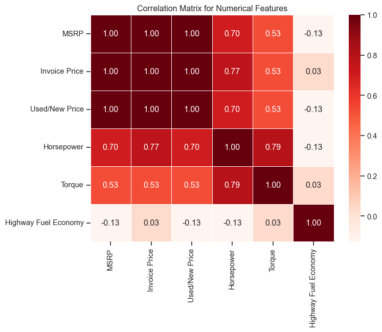
I am taking out correlated columns whose correlation to MSRP is exactly 1.
After Handling Correlation: Columns are…
numerical_cols = ['MSRP', 'Horsepower', 'Torque', 'Highway Fuel Economy']

categorical_cols = ['Make','Year', 'Body Size', 'Body Style',
                    'Cylinders', 'Engine Aspiration', 'Drivetrain',
                    'Transmission']
4. Remark
Data cleaning is an ongoing process. As we conduct further analysis, such as data visualization and storytelling, additional issues, including outliers, may emerge. However, at this stage, we have completed the initial phase of data cleaning.
Columns that made it
numerical_cols = ['MSRP', 'Horsepower', 'Torque', 'Highway Fuel Economy']

categorical_cols = ['Make','Year', 'Body Size', 'Body Style',
                    'Cylinders', 'Engine Aspiration', 'Drivetrain',
                    'Transmission']
5. Save Data
# Define numerical and categorical columns
numerical_cols = ['MSRP', 'Horsepower', 'Torque', 'Highway Fuel Economy']
categorical_cols = ['Make', 'Year', 'Body Size', 'Body Style',
                    'Cylinders', 'Engine Aspiration', 'Drivetrain',
                    'Transmission']

selected_cols = numerical_cols + categorical_cols
cleaned_df = df[selected_cols]

# Save the cleaned dataset to a CSV file
cleaned_df.to_csv("cleaned_data.csv", index=False)

print("Cleaned data saved as 'cleaned_data.csv'.")
Cleaned data saved as 'cleaned_data.csv'.
Next Steps
Now, you can move to the next notebook, where I perform exploratory data analysis (EDA) to gain insights.